Attention Is All You Need: In-Depth Walkthrough

In this blog post, I will walk through the “Attention Is All You Need,” explaining the mechanisms of the Transformer architecture that made it state-of-the-art.

The Transformer. Attention Is All You Need Figure 1.

The goal is to understand why the Transformer was so groundbreaking and how it achieves these capabilities by implementing each part manually, relying only on NumPy without any out-of-the-box packages from Keras or PyTorch.

Being a deep-learning beginner myself, I will try to add as much depth as possible to explain the author’s design choices since the original paper assumed a lot of implicit background knowledge that may not have always been apparent to novices. Hence, this post is best suited for beginners who have a basic understanding of machine and deep learning concepts and general linear algebra (vectors and matrix multiplication).

The post will be split up into three parts:

• Why the Transformer architecture was so groundbreaking

  • First, I will introduce some background information on the state of sequence modeling at the time the paper was published in 2017 and the challenges that these models faced.

• How the Transformer architecture is structured

  • Then, I’ll give a holistic overview of the Transformer architecture to how the Transformer architecture and attention mechanism overcame these challenges from a high level.

• Deep dives into individual parts of the Transformer with implementations

  • Lastly, I’ll dive into each respective part of the architecture to build an intuitive understanding of the author’s design choices and how these actually address the challenges.

What I will not touch upon is an actual working implementation of the Transformer. This would require additional focus on general model training best practices that for example consider batching, warm-up, parameter fine-tuning, and packing the functionalities into trainable layers. My goal is to present the mechanisms as pure as possible – not necessarily in the most reusable and efficient manner.

Why the Transformer architecture was so groundbreaking

To build an intuitive understanding of why the paper and the proposed model architecture became so influential for state-of-the-art deep learning models, we have to first get a feeling for where sequence modeling was when the authors published the paper.

At the time, Recurrent Neural Networks (RNNs) were the standard for sequence-to-sequence modeling, especially in the Natural Language Processing (NLP) domain. Through their recurrent structure, they were able to capture sequential meaning which is essential in understanding our language and in turn, translation and text generation tasks. I will not dive into the architecture of RNNs here and assume that the reader already knows how RNNs work (if not check out this resource). They were able to be trained on large bodies of text and achieve great performance in translation and next-word prediction tasks.

However, they also came with challenges that had yet to be solved. Downsides included:

• Long training times: Due to processing information sequentially and predicting elements in sequence based on all the previous elements, the model could not utilize parallelization when being fed an input. They were still able to train on multiple inputs at a time but for a single input, the model had to process each element in the input sequence step by step. This did not allow the RNNs/ LSTMs/ GRUs to use parallel computing hardware like GPUs which was crucial for efficient training and use of computation resources.

• Difficulties with capturing long-range dependencies: An important aspect of modeling language is capturing how words relate to each other. RNNs store these connections in hidden states that get updated with each new input. This works well when the sequence is short. When the range of a dependency between elements of a sequence is very large, the connection between words, however, could get lost because too many recurrent layers would have to be involved, creating the vanishing or exploding gradient problem (will not be explained here, for details check out this). This was even the case for LSTMs and GRUs which were meant to combat the general RNNs’ downsides. Ultimately, the sequential nature of the models made both training and performance on long sequences difficult.

In summary, what made sequential models good for capturing semantic context in sequences introduced computational efficiency issues.

In contrast to these parallelization issues, we had Convolutional Neural Networks (CNNs) and specifically Residual Networks (ResNets) which took full advantage of computational parallelization. I will also not dive into the actual architecture of CNNs here and assume general knowledge of these.

In the deep dive, however, I will discuss ResNets more in detail in case the reader is not familiar with these yet. In general, CNNs and ResNets were able to:

• Apply convolution simultaneously: By having kernels and convolution functions, they could apply the same convolution over an entire image in parallel which drastically reduced training time.

• Train very deep models: The ResNet architecture introduced so-called residual connections which allowed backpropagation to skip out on groups of layers when no additional information was actually gained from these. This process effectively reduced the issue of vanishing and exploding gradients. More about this later on.

So while sequential models had issues there were other model architectures that already effectively combatted them.

In addition to convolution and recurrence, attention as a mechanism to learn about relationships of elements in a sequence already become integral for sequence modeling given their ability to disregard the actual distance between elements in a sequence. However, there weren’t many models that fully abandoned recurrent structures even when using attention which meant that they still had to deal with computational issues.

With this background information, it should have become clear that solving the RNNs downsides could be possible. This is exactly what the authors of “Attention Is All You Need” did. They combined the best of RNNs, ResNets, and the attention mechanism to construct a new Transformer architecture that not only successfully removed parallelization bottlenecks but also outperformed existing state-of-the-art models in translation.

How the Transformer architecture is structured

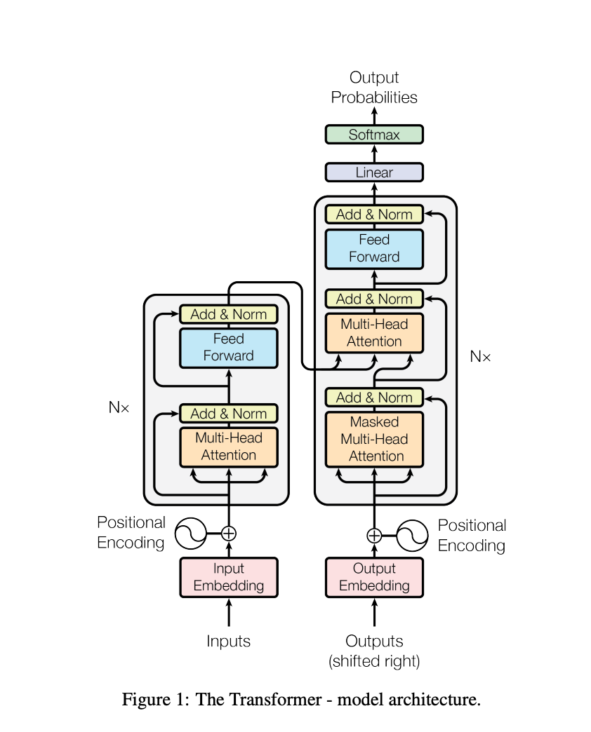
As described in the previous section the Transformer architecture combines attention with ResNet functionality using the coming decoder-encoder structure that is often used in LSTMs for language translation and generation tasks. From a very high-level perspective, the architecture can be summarized as the following: A large Encoder layer with attention, a large Decoder layer with attention, embeddings, and positional encoding.

Abstracted Transformer Architecture. From heiswicked.log.

Before any data enters the Transformer, it gets embedded. Embedding represents a vectorized version of a token that stores information about the word across various dimensions. A token in turn represents an element in a sequence – usually a word in a sentence. 

The embedded version of the words also gets enriched with information about where the word is located in the sequence or sentence. This is called Positional Encoding.

The Encoder uses the positionally embedded version of a source language (for example English in an English-to-German translation task) as input and tries to generate an enriched version also called a representation of the source that captures more than just the words themselves: semantic meaning, relationships, order, implicit meaning. Think of these representations as annotations – each word gets annotated with a lot of additional information and context.

The Decoder uses a fraction of the positionally embedded target language (for example only the first half of the sentence of the translated English sentence in German) in combination with the enriched representation of the source language to predict which German word to use next to effectively translate the English sentence.

It is important to note that the Encoder never has access to any information from the Decoder but the Decoder has access to the Encoder – this constitutes the core mechanism of a decoder-encoder structure.

Within the Encoder and Decoder, there are sublayers that help with the final rich representation of the source and target. The Encoder has two sublayers: an attention and a Feed Forward layer (more in detail later). The Decoder has an additional sublayer, making it two attention layers and one Feed Forward layer.

Both the Encoder and Decoder layer employ attention mechanisms as part of their sublayers which allows both layers to learn about dependencies within a source or target sequence.

This high-level overview serves as a starting point and guide for the next deep dive into each part of the Transformer. If you should feel lost during this deep dive, refer back to this section to understand where we are currently at and what the larger picture looks like.

Deep dives into individual parts of the Transformer with implementations

We will walk through each part of the Transformer model in order from start to finish. As part of each deep dive, we will process an example in Python and explain how the example changes to build an intuitive understanding of the Transformer’s mechanisms.

Each section will have a Description part that explains and describes the Transformer subcomponent.

Additionally, you will find an Implementation part showing how the layer would be implemented as a simple Python function as well as an Example output that applies the implementation and returns the new representation of the original input.

Note: The code implementation will only represent a forward pass, meaning that no training actually takes place and, thus, predictions will be entirely inaccurate. The goal is to get an intuitive understanding of the mechanisms. An actual trainable model may be implemented in a separate post using PyTorch’s modules.

Input

Description

As mentioned in previous sections, Transformers help with sequence-to-sequence tasks and are fed corpora of text to learn the underlying structure and patterns of our language. They are often trained on billions of data points through text crawled from the internet.

In the context of language translation, the Encoder receives the source language.

Throughout the deep dive we will use the following sentence and it’s translation to follow each transformation step:

The cat didn't cross the street because it was too wide.

Implementation

We store the sentence in a list since the Transformer processes one sentence at a time. Usually, we would store a larger corpora of text and process them in parallel. For the purpose of the example, we will only use one sentence.

We also have to add a <end> token to give the embedding a unified signal for when a sequence ends.

input = ["The cat did not cross the street because it was too wide <end>"]

Input Embedding

Description

The architecture starts with an input embedding. Embeddings are also the base of many CNNs and RNNs and as such don’t necessarily represent a new mechanism.

Embeddings in the context of NLP convert words into vector representations that capture additional semantic meaning. In this case, the Embedding unit generates a 512-dimensional vector where each dimension abstractly stores some information about a token.

---

Note: Throughout the entire model, the Transformer keeps the data’s dimensionality to 512 dimensions in almost all instances. This will not be explicitly reiterated but carefully considered in any code implementation.

---

In the original paper architecture, the embedding itself gets learned but there is no additional information about the used embedding model. Given that embedding is not the core focus and is an already existing mechanism, we will use ELMo to represent these embeddings WITHOUT learning. In the complete Transformer architecture, we would also learn the parameters of the input embedding layer.

Embedding Example.

Implementation

We import ELMo as a pre-trained embedding model. Since ELMo embeds tokens as 1024-dimensional tensors and the Transformer operates in a 512-dimensional space, we have to project the embeddings back to a 512 vector.

Example Output

Positional Encoding

Description

One big advantage of sequential models is the ability to extract information about the order of words. However, because sequential processing through recurrence limits parallelization, a different mechanism needs to be employed. For this, the Transformer uses Positional Encoding which can be applied to all positions simultaneously.

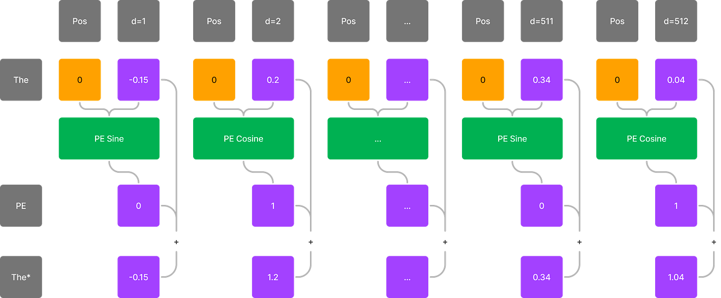
Positional Encoding takes the position of a token in sequence, encodes it in a richer representation similar to the embedding itself, and adds that representation to the original embedding. Adding here means either through mathematical addition or horizontal concatenation.

In the paper, the authors decided to use two deterministic functions to store the position with addition instead of concatenation. Since the original embedding vector has 512 dimensions the positional encoding also generates a 512 dimensional vector with positional information spread out across the 512 dimensions. 

To capture information as rich as possible, they used a sine function for odd dimensions and a cosine function for even dimensions.

Positional Encoding functions.

Why two functions and why sine and cosine?

There were many options but the authors seem to have empirically decided that this option for Positional Encoding would provide as much unique positional information as possible. Uniqueness is key here since storing redundant information reduces the potential relationships that can be learned.

Positional Encoding example.

Using sinusoids and specifically sine and cosine has multiple benefits:

• The goal of Positional Encoding is to teach the model to learn the relativity between two positions. Thus, the Positional Encoding functions need to express relativity between positions well enough. Sine and cosine shifts can be represented by a linear function of sine and cosine using trigonometric identities. 

\(\sin(x + k) = \sin(x)\cos(k) + \sin(k)\cos(x)\)

\(\cos(x + k) = \cos(x)\cos(k) - \sin(a)\sin(b)\)

For a specific difference k in position, sine and cosine can represent this shift explicitly.

• Cosine is sine shifted by one π, thus, always representing the exact opposite of sine. By having two functions that are in contrast to each other they ensure that dimensions store all potential representations of the position without repeating any information, avoiding redundancy.

• Sinusoids stretch infinitely and are repetitive. This is very beneficial for storing very long sequences.

Sine gets applied to 2i while cosine gets applied to 2i+1 – values can alternate between odd and even dimensions.

Inside the sine and cosine function the frequency of the wave is determined by the denominator. Since d_model is a constant, only the dimension affects the denominator and as such the frequency of the sinusoids. This means that each dimension can represent the position at a different frequency. These different frequencies allow the model to learn positional differences in various representations.

Another option would have been to use a learnable Positional Encoding function instead of fixing it with a deterministic function. The authors also tested a learned function but decided to use a fixed one for the Transformer architecture since this reduces the number of parameters and improves computation.

Implementation

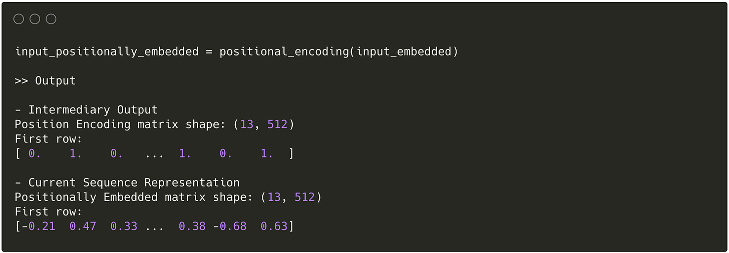
For each row in the matrix (representing a word vector), we iterate through each dimension and calculate the positional encoding using both the row index and dimension index.

Example

Encoder

The Encoder represents one of the two main parts of the Transformer architecture. Although the general encoder-decoder structure was not completely new during the time the authors published the paper, the sublayers within the Encoder and Decoder gave the architecture its unqiue capabilities.

Using the positionally augmented embeddings as input, the Encoder processes the information through two sublayers:

• The first sublayer applies the attention mechanism through a so-called Multi-Head Attention unit.

• The second sublayer consists of a position-wise Feed Forward fully connected network that we already know from simple Multi-Layer Perceptrons.

Let’s dive into each part.

Multi-Head Attention

The multi-head attention layer combines two parts: multi-head and attention. We’ll first discuss the attention piece and then connect it with the multi-head mechanism.

Attention Is All You Need Figure 2.

Attention

Description

To understand why the authors decided to implement an attention mechanism we have to take a step back and remind ourselves of the initial purpose of the Transformer architecture:

• To overcome the computational inefficiencies in recurrent structures,

• And capture more long-range dependencies.

For that, attention had to not only capture more context than sequential processing but also be parallelizable. Keeping this in mind, we can now dive into the actual mechanism and implementation.

Attention, in a nutshell, means how much an element in a sequence should be considered in the context of the other elements in the sequence.

Let’s take our original sentence example: "The cat didn't cross the street because it was too wide."

Attention Example.

Although this sentence may be poorly constructed because of the ambiguity of “it,” being proficient in English, we know that “it” can only refer to the street because a “too wide” cat would not make sense (well in some abstract sense it could but we wouldn’t refer to a cat as wide …). We pay attention to “too wide” to understand what “it” means and what the word is referring to. In an attention mechanism, the model would learn to pay attention to “too wide” to understand the meaning and use of “it”.

This sounds quite straightforward but how do we actually represent this attention functionality in code, make it parallelizable, and at the same time allow it to capture more long-range dependencies? As with anything in machine learning through weights and matrices or as the authors called it: Scaled Dot-Product Attention.

Scaled Dot-Product Attention

Scaled Dot-Product Attention consists of two mechanisms, scaling and performing a dot-product. We will take a look at the dot product first.

Dot-Product 

Conceptually, when considering how attention within a sequence works, we are essentially trying to understand how much a specific token’s meaning depends on the other tokens in the sequence.

This can represented by a function where we input a token of a sequence and get back a score for each other token in the sequence – the attention score. For this function, each token gets attention from the other tokens, helping to provide meaning to other tokens, and gives attention, gathering meaning from other tokens.

Attention Function example.

There are various ways to represent this attention function and the main ones implemented in models are additive attention and multiplicative attention. What makes these forms of attention special is the ability for each token to compute attention scores with every other token in the sequence directly. This means that dependencies between any two tokens are just one step away in a computational graph, regardless of their position in the sequence. Additionally, because the path lengths between positions become constant, processing can happen simultaneously for all tokens in a sequence. In contrast, LSTMs process sequences step-by-step, which requires an additional recurrence for each additional distance step.

The authors chose multiplicative or dot-product attention and constructed this function through a multi-step process that incorporates Queries, Keys, and Values (which has become state-of-the-art for the majority of LLMs today).

In their setup, the input element plays three roles:

• As a “query” that asks the other tokens how much attention the query token should pay to the other tokens (“keys”).

• As a “key” so that when a “query” asks for how much attention it should pay to the input token, it can respond.

• As a “value” that determines what content of the token should contribute to.

Transformer Attention. From Sebastian Raschka.

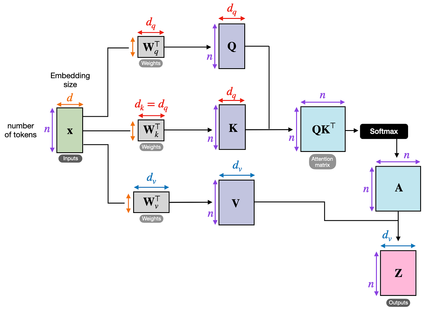
Each of these roles is accompanied by weight matrices that create a different representation of the original input vector specific to the role they take on. With these roles established, we can finally compute the actual attention by combining each token’s query identity with each other token’s key identity through the dot-product.

For a specific “query” (selected token) and “keys” (all other tokens), we use the dot-product to approximate attention. The dot-product in linear algebra is used to calculate how similar two vectors are, where similarity ranges from very negative to very positive numbers constrained by the vector’s “length” (for a deep dive into the dot-product, I suggest this article). Although attention doesn’t mean that two words are similar, we can use similarity to approximate attention. By having previously added the role-specific weight matrices we introduced a way for the model to tweak the weights so that the dot-product actually represents attention instead of similarity. We will call the output of this step the raw attention weights.

Before we use these raw attention weights to construct a representation of the original token as a combination of all the other tokens – a weighted sum – we have to apply some additional transformations to ensure that the weights can be well used and trained by the model.

Scaling

In the original figure, there is an additional masking operation which we will skip for now as this is only relevant for the Decoder.

To ensure that the raw weights can be effectively used, we have to introduce additional non-linearity and normalization. For this purpose models often use the SoftMax function which translates raw weights or logits into values between 0 and 1 that sum to 1. The SoftMax function is a standard activation function in machine learning so we will not dive deeper into the specificites. For more details on SoftMax check out this definition.

The SoftMax function is sensitive to the actual numerical number of the raw weight due to the exponentiation of values. Large raw values dominate smaller values, making the training much more difficult because the few large values will be close to 1 while all other values are pushed to be close to 0. In addition, there are also stability considerations where the actual underlying computation could lead to overflow when numbers are too large.

To mitigate this, Scaling is used. The raw attention weights are scaled by dividing by the square root of the dimension of the key vectors (we will get to dimensionality later during the Multi-Head discussion).

Continued Dot Product

With the scaled and soft-maxed weights, we can now calculate a representation of the input vector that uses the attention weights to determine how much it should be composed of the other vector’s values. For this, we apply another matrix multiplication but in this case, it represents a  weighted sum of all the value vectors.

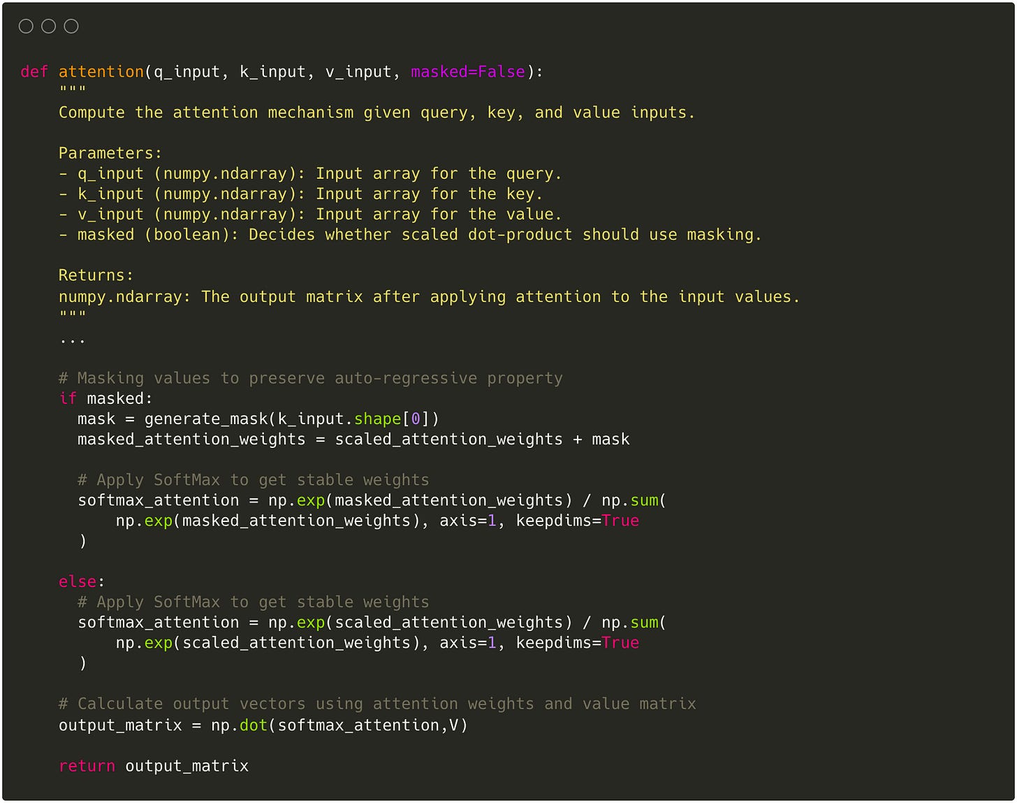
Implementation

For Q, K, and V we have to create a learnable weight matrix in the form of a Dense Feed Forward layer with linear activation.

Once the query, key, and value matrices have been generated through the linear projection, we take the dot product between Q and K and apply scaling and softmax.

The final normalized weights can then be multiplied with the value matrix to get each word represented as the weighted sum of all other words according to the attention weights.

Example

Multi Head

Description

Now that we know how the attention mechanism works in practice, we can turn our attention to the Multi-Head aspect. For this, we need a quick side tangent: One ground principle in machine learning is the goal to capture as many patterns and relationships between individual data points as possible. This can be achieved by transforming data in many different ways and assessing whether the transformed version uncovers relationships that wouldn’t be apparent by just one representation of the data. Initially, the new transformed representations may be uninsightful but over time the model learns to create representations that help with its task.

Multi-Head Attention example.

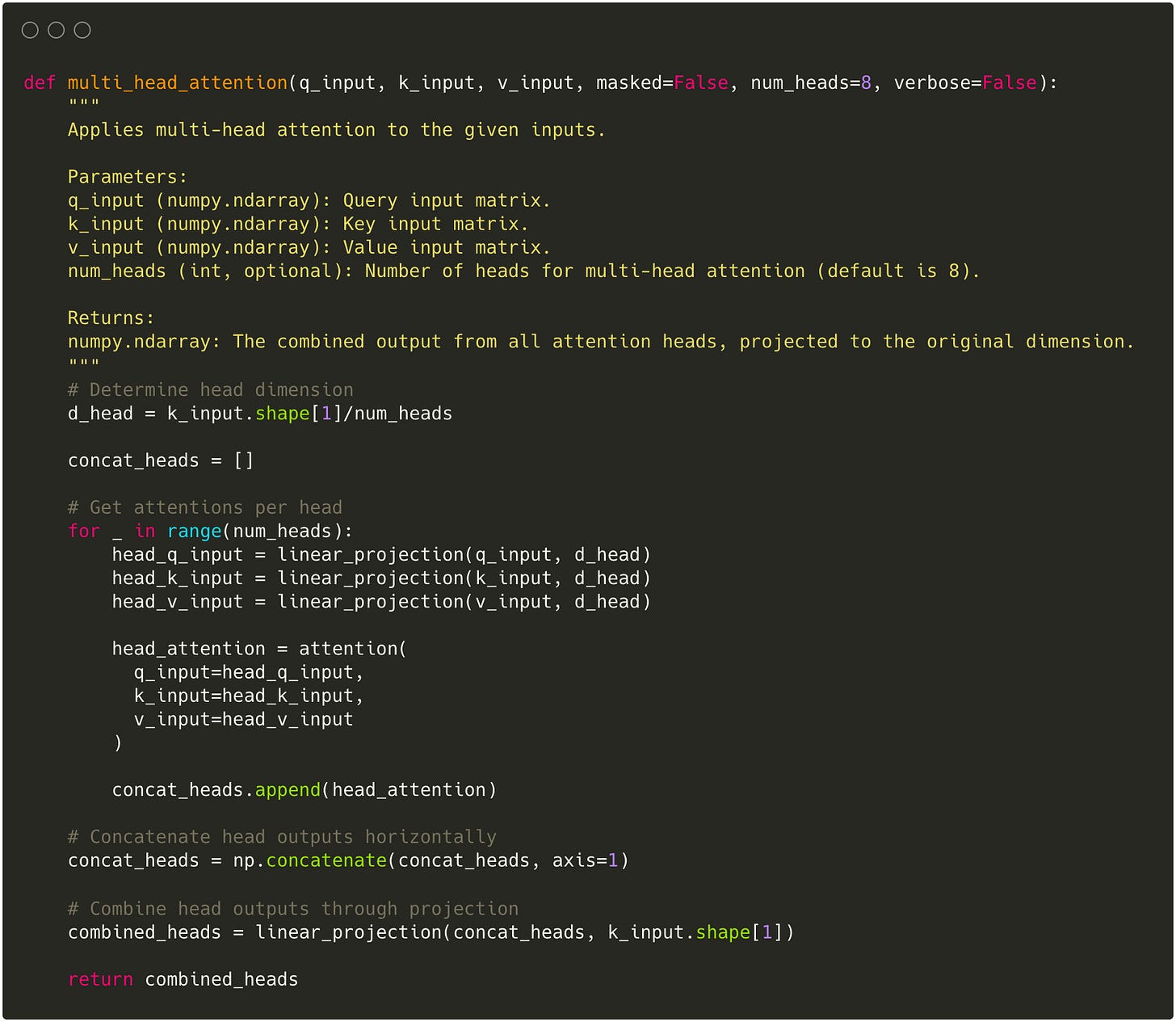
The multi-head concept enables this principle by replicating the attention mechanism multiple times where each version of the attention mechanism can learn to pay attention to other characteristics. Each of these attention mechanisms, or “head”, has its own sets of parameters that get randomly initialized and, thus, have a different starting point. This difference in initialization allows the model to learn different attention representations.

One downside of the Multi-Head approach is the addition of parameters since more heads also mean that more parameters have to be learned. To mitigate this, each head in the Transformer gets scaled down to a fraction proportional to the number of heads of the original dimensions so that the computation is similar to just having one large head.

To bring it all back together, after each head calculates the final weighted value vector they all get horizontally concatenated and combined through a linear linear so that each individual’s head’s information gets passed most effectively for further sublayers.

With this, we have covered the main functionality of the Transformer that implements attention in a way that allows parallelization. 

Implementation

Based on the desired number of Heads, we adjust the dimensions of each Head and generate the output vector using the attention function.

Each Head’s output gets horizontally concatenated and again projected to combine each Head’s information into one representation.

Example

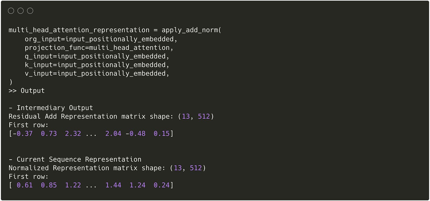
Residuals and Normalization

Residuals

Description

Although parallelization and long-range dependencies were majorly already solved by the Multi-Head Attention sublayer, the model would still face issues if many of these layers were stacked on top of each other due to the vanishing gradient problem. Thus, next in line after the multi-head attention we have the addition and normalization layer.

The addition represents a residual mechanism that we touched upon in the introduction when talking about CNNs and residual networks. Residual networks introduce skips in the network where instead of continuing only with the newly represented vector, which could become purely noise, the model adds the original vector to the new representation of the vector. Through this, the model does not only learn the new representations but also how these relate to the original representation. For example, if the representation should not be helpful at all, the model may decide to learn an “identity mapping” instead, essentially just taking the original input as is with a bit of noise instead of having to consider the new representation in downstream layers.

Residual Addition mechanism. From Wikipedia.

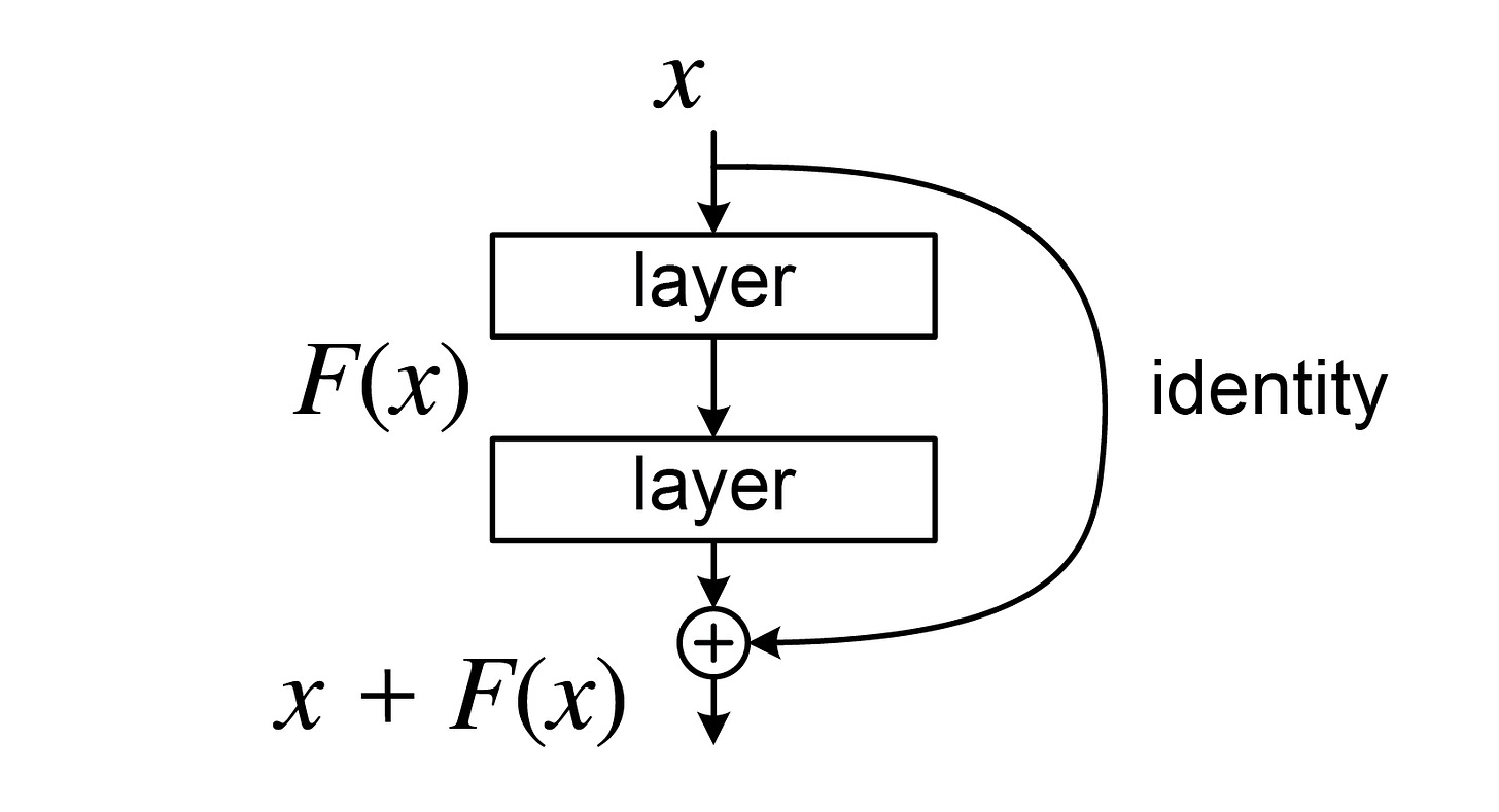
Without the residual mechanism, deep networks would struggle to effectively learn because after layers and layers of projection, we often times end up with representations that almost only look like noise. Training on this noise becomes difficult for very deep networks. With these residuals, the model gets shorter learning path so that when the representations are not as insightful in the beginning we can still propagate learning across layers effectively by skipping out on the sub-layers and later on, when the sub-layers have learned relevant representation, then learning can continue to be effective within sub-layers.

To achieve this residual effect, values are either added to the original vector or concatenated similar to the multi-head attention scenario. For adding, dimensionality needs to remain consistent while for concatentation dimensionality doesn’t matter but more parameters get introduced. In this paper, the authors chose to use adding instead of concatentation to avoid learning more parameters which also introduced the requirement to keep the output of all layers consistent to 512 dimensions.

Implementation

Normalization

Description

After adding the residuals the model applies normalization which centers the values across dimensions around 0 and scales the values accordingly. There are multiple benefits around preserving stability and learning, improving generalization by adding noise, and accelerating training. Given how common this mechanism is within the context of machine learning models, I will not dive deeper into the actual reasoning. For further information on normalization check out this.

The residual and normalization layer gets applied as part of each sublayer so I will not explicitly mention them each time. 

Implementation

Since the same add and norm layer gets applied multiple times, we make it a more generic function.

Example

Feed Forward

Description

As the last core sub-layer in the encoder, we have a feed-foward network (FFN) that consists of a hidden layer with ReLu activation. What’s special about the FFN implementation here is that the same FFN gets applied to each position, thus being a position-wise FFN. Although the FFN gets applied to each position, the FFN shares the same parameters for all positions so all positions affect how the FFN adjusts its weights. Again, because FFNs are foundational to any machine learning, I will not dive into the FFN’s specifics.

In essence, they introduce non-linearity through the ReLu activation function, increase representation power by projecting the normalized output vectors into a higher dimensional space, in the case of the paper to a 2048 dimensional vector, and get to learn an effective representation that captures both attention and position-related information. Since the FFNs are point-wise, they can be trained in parallel.

Implementation

Example

Feed Forward only output.

That’s it – that’s how the Encoder works. Next up, we will dive into the Decoder which in many parts looks just like the Encoder.

Outputs

As mentioned in the general overview section, a decoder-encoder structure relies on the Encoder to learn about the source language and the Decoder to learn about the target language. Thus, the Decoder receives the target language or our desired output as its input.

Instead of feeding the target language to the Embedding Layer in full like we did in the Encoder architecture, the outputs get shifted to the right with a padding start element. This ensures, that the last element is not accessible to the model which teaches the model to predict the next element in the sequence given the previous elements. This supports the preservation of the so-called auto-regressive property which ensures that a model only generates tokens of a sequence conditioned on the previous tokens it has generated and seen.

Le chat ne a pas traversé la rue parce que elle était trop large.

# Removing the last element and padding a start element
output = ["<start> Le chat ne a pas traversé la rue parce que elle était trop"]

Output Embedding

Similar to the Encoder, outputs get embedded into higher dimensional vectors. The Output Embedding does not share parameters with the Input Embedding, meaning that both Embeddings are learned. For the sake of this walkthrough, we will not dive into this part of the embedding either and use the ELMo embedding model again without any training.

Positional Encoding

The exact same mechanism for Positional Encoding gets applied here, adding positional information to the embedded vectors.

Decoder

The Decoder represents the second main part of the Transformer architecture. It is almost identical to the Encoder architecture except with an additional sub-layer that is used to prevent the Decoder from accessing information about tokens in the sequence that it is not supposed to know about yet.

The Decoder first learns about the already generated output using a Masket Multi-Head Attention Layer on the embedded target sequence alone, then combines the learned representation with what it already has learned about the source sequence’s structure and semantics in a second Multi-Head Attention sublayer, and finally returns a representation of the next word which gets mapped back to the actual target language vocabulary.

This structure allows the Decoder to use both the semantics in the source and target language to come up with a context aware prediction in the target language.

Just like in the Encoder, residual addition and normalization also gets applied after each sub-layer to retain the advantages described in the Encoder section.

Masked Multi-Head Attention

Description

As mentioned in the Multi-Head Attention part of the Encoder, there is a Masking part that we will address as part of the Decoder.

In addition to shifting the data to the right by one index, the Transformer also needs to ensure that at any position, no future tokens get considered or paid attention to. For that, we set all positions after the current to negative infinity which returns a zero probability after applying SoftMax.

Since the masking gets applied after the raw attention weights get computed we can simply use an upper triangular matrix with NxN dimensions and -inf for any value above the diagonal that we add right before we apply SoftMax in the Scaled Dot-Product Attention.

Masking mechanism. From Revistek.

Apart from that, we use the same mechanism as described in the Encoder but instead on the masked target (output) language vectors. This allows the Decoder to learn attention in the target language which can be used for the next word prediction.

Implementation

Generates upper triangle mask.

Adding masking functionality before applying SoftMax to the previous attention function.

Adding masking functionality to Multi Head Attention mechanism.

Example

Masked single-head example with masking.

Masked multi-head example.

Multi-Head Attention

Description

Until now, there has been no interaction with the Encoder’s output to inform the Decoder about the learned context that can be used for the next word prediction. For this, a regular Multi-Head Attention layer is stacked on top of the masked version using the output of the Masked Multi-Head Attention as queries for the Query matrix and the output of the Encoder as keys and values for the Key and Value matrix – a process called encoder-decoder attention.

Decoder-Encoder Attention example.

Here, the Decoder calculates attention based on the representation of the target language tokens and the Encoder’s representation of the source language tokens (called context vectors). Through this, the Decoder gets informed about the source sequence with all of its rich representation to then generate a representation of the output elements that can be used to predict the next word.

Again, due to the Scaled Dot-Product Attention, each position in the Decoder directly and simultaneously accesses all positions in the Encoder – enabling parallelization and long-range dependency representation also across the Decoder and Encoder.

After combining both the Decoder and Encoder representations, another point-wise FFN layer creates a final representation similar to the Encoder. Here, the Decoder’s FFN does not share parameters with the Encoder’s FFN.

Example

Linear

Description

Once the final representation has been added to the original output from the Feed Forward sublayer and normalized. A linear transformation is applied through a fully connected neural network layer that maps the representations back as logits to the original vocabulary list. Each neuron in this layer corresponds to one word in the vocabulary.

Implementation

We use the same linear projection function with the original vocabulary size to return a matrix with dimensions n x vocab_size.

Example

SoftMax

Description

To get the actual probabilities for each word in the vocabulary a final SoftMax is applied which turns the logit values into probabilities between 0 and 1 which sum to 1. These probabilities are then used to predict the target next word.

Example

Here, the probability of the first position would be the fifth word.

Additional Architecture Details

In addition to the core architecture already outlined, the Transformer extends the sublayer set by stacking multiple Encoders and Decoders on top of each other which adds even more potential representations of relationships.

There are 6 Encoders stacked on top of each other, using the previous Encoder’s output as the input.

There are also 6 Decoders stacked on top of each other, also using the previous Decoder’s output as the input in addition to the final Encoder’s output within each individual Decoder’s multi-head attention layer.

The individual Encoders and Decoders do not share any parameters, thus, adding 6 times the parameters in total.

End-to-End Example

To fully see how inputs get processed, projected, and transformed into new representations, we will use a simple example and reduce the model dimensions to 6.

Source Input: I am a student.

Target Output: Je suis étudiant.

To view each individual transformation explore the following FigJam which walks through all steps and shows how the first row would be transformed in a forward pass for only one Encoder and Decoder layer: FigJam Diagram.

Full Transformer Example

Wrap Up

There is additional detail about the actual training of the model in the paper which we have not touched upon yet. This may be part of a second post as this post was primarily dedicated to understanding the architecture of the Transformer first. This also means that any Python implementation does not actually represent a trainable model yet since they all have to be tied together and constructed as layers of a model to apply a learning algorithm that updates each individual layer.

---

Resources: Attention Is All You Need

Code: Simple Transformer Implementation in Python